What Happens To Costs As Output Increases?

Learning Objectives

Identify economies of scale, diseconomies of scale, and constant returns to scale

Before in this module nosotros saw that in the short run when a firm increases its scale of performance (or its level of output), its boilerplate toll of production tin can decrease or increase. This is illustrated in Figure one.

A u-shaped curve.

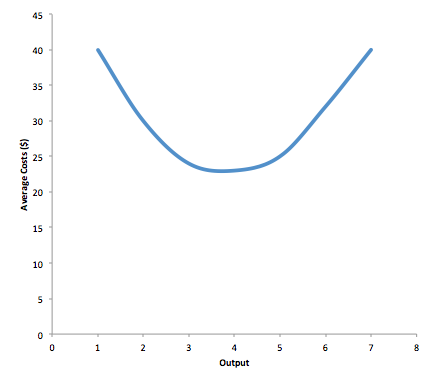
Figure i. Short Run Average Costs.The normal shape for a curt-run boilerplate cost curve is U-shaped with decreasing average costs at low levels of output and increasing average costs at high levels of output.

What happens to a business firm's average costs when it increases its level of output in the long run? Many industries feel economies of calibration.Economies of scale refers to the situation where, every bit the quantity of output goes up, the cost per unit of measurement goes down. This is the idea behind "warehouse stores" like Costco or Walmart. In everyday language: a larger factory can produce at a lower average cost than a smaller factory. Figure 2 illustrates the idea of economies of scale, showing the boilerplate cost of producing an alarm clock falling equally the quantity of output rises. For a small-sized manufactory like S, with an output level of i,000, the average cost of product is $12 per alert clock. For a medium-sized manufacturing plant like M, with an output level of ii,000, the average cost of product falls to $eight per alarm clock. For a large manufactory similar L, with an output of 5,000, the boilerplate cost of product declines notwithstanding further to $four per alarm clock.

The graph shows a downward sloping line that represents how large-scale production leads to a decrease in average costs.

Figure 2. Economies of Scale A pocket-size factory like Due south produces 1,000 alarm clocks at an boilerplate price of $12 per clock. A medium factory like M produces 2,000 alert clocks at a toll of $viii per clock. A big factory like L produces 5,000 alarm clocks at a price of $4 per clock. Economies of scale exist because the larger scale of production leads to lower average costs.

The average price curve in Figure two may appear like to the boilerplate cost curve in Figure 1, although it is downward-sloping rather than U-shaped. Merely there is one major deviation. The economies of scale bend is a long-run average toll bend, because it allows all factors of product to alter. Curt-run average cost curves assume the existence of fixed costs, and only variable costs were allowed to change. In sum, economies of scale refers to a situation where long run average cost decreases equally the firm'southward output increases.

One prominent example of economies of scale occurs in the chemical industry. Chemical plants take a lot of pipes. The price of the materials for producing a pipe is related to the circumference of the pipe and its length. Even so, the volume of chemicals that can flow through a pipe is determined by the cross-section surface area of the pipage. The calculations in Table 1 show that a pipe which uses twice as much material to brand (every bit shown past the circumference of the pipe doubling) can actually carry iv times the book of chemicals considering the cross-department area of the pipe rises by a cistron of four (as shown in the Area column).

Table 1. Comparing Pipes: Economies of Scale in the Chemical Industry
	Circumference ( ii π r )	Surface area ( π r 2 )
four-inch pipe	12.5 inches	12.5 square inches
8-inch pipage	25.1 inches	fifty.2 square inches
xvi-inch pipe	50.2 inches	201.1 square inches

A doubling of the cost of producing the pipe allows the chemical business firm to process four times as much textile. This pattern is a major reason for economies of calibration in chemical product, which uses a big quantity of pipes. Of course, economies of scale in a chemical plant are more complex than this simple calculation suggests. Only the chemical engineers who design these plants have long used what they call the "six-tenths dominion," a dominion of thumb which holds that increasing the quantity produced in a chemical plant by a certain percent volition increase total price by only six-tenths as much.

Sentinel It

Watch this video to see an example of economies of scale as practical to making bread.

Shapes of Long-Run Average Cost Curves

While in the short run firms are limited to operating on a single average cost curve (corresponding to the level of stock-still costs they take chosen), in the long run when all costs are variable, they can choose to operate on any average price curve. Thus, thelong-run boilerplate cost (LRAC) curve is really based on a grouping of short-run average toll (SRAC) curves, each of which represents one specific level of fixed costs. More precisely, the long-run average cost bend volition be the least expensive average toll curve for whatever level of output. Figure 3 shows how the long-run average toll curve is built from a group of short-run boilerplate toll curves.

Five short-run-boilerplate cost curves appear on the diagram. Each SRAC curve represents a different level of fixed costs. For example, you can imagine SRAC₁ as a small mill, SRAC_ii as a medium manufacturing plant, SRAC₃ as a large factory, and SRAC₄ and SRAC_v as very big and ultra-big. Although this diagram shows only 5 SRAC curves, presumably there are an infinite number of other SRAC curves between the ones that nosotros show. Retrieve of this family unit of curt-run boilerplate toll curves as representing different choices for a house that is planning its level of investment in fixed cost concrete capital—knowing that different choices about uppercase investment in the present will crusade information technology to end upwardly with different short-run boilerplate price curves in the future.

This graph shows a long run average cost as a sum of minimum short run average costs.

Figure 3. From Curt-Run Average Price Curves to Long-Run Average Price Curves The five different short-run average cost (SRAC) curves each represents a different level of fixed costs, from the depression level of fixed costs at SRAC₁ to the high level of stock-still costs at SRAC₅. Other SRAC curves, not shown in the diagram, prevarication between the ones that are shown hither. The long-run boilerplate cost (LRAC) bend shows the lowest toll for producing each quantity of output when fixed costs can vary, and so it is formed past the bottom border of the family of SRAC curves. If a firm wished to produce quantity Q_iii, it would choose the fixed costs associated with SRAC₃.

The long-run average cost curve shows the cost of producing each quantity in the long run, when the house can choose its level of fixed costs and thus choose which short-run average costs information technology desires. If the business firm plans to produce in the long run at an output of Q₃, it should make the set of investments that will atomic number 82 it to locate on SRAC_iii, which allows producing q_three at the lowest cost. A firm that intends to produce Q₃ would exist foolish to choose the level of fixed costs at SRAC₂ or SRAC₄. At SRAC_two the level of fixed costs is too low for producing Q_iii at lowest possible price, and producing q₃ would require adding a very high level of variable costs and brand the boilerplate toll very high. At SRAC₄, the level of fixed costs is besides high for producing q₃ at everyman possible toll, and once more boilerplate costs would be very high as a result.

The shape of the long-run toll bend, in Figure three, is adequately common for many industries. The left-hand portion of the long-run average cost curve, where it is downward- sloping from output levels Q₁ to Q_two to Q_iii, illustrates the instance of economies of calibration. In this portion of the long-run average toll curve, larger calibration leads to lower average costs. We illustrated this pattern earlier in Figure ii.

In the center portion of the long-run average cost curve, the flat portion of the curve around Q₃, economies of calibration have been wearied. In this situation, allowing all inputs to expand does non much alter the boilerplate cost of production. Nosotros phone call this constant returns to calibration. In this LRAC curve range, the average cost of product does not change much every bit calibration rises or falls.

How do Economies of Scale Compare to Diminishing Marginal Returns?

The concept of economies of scale, where boilerplate costs turn down as product expands, might seem to disharmonize with the thought of diminishing marginal returns, where marginal costs rise as production expands. But diminishing marginal returns refers only to the short-run boilerplate cost curve, where one variable input (similar labor) is increasing, but other inputs (like uppercase) are stock-still. Economies of calibration refers to the long-run average cost curve where all inputs are being allowed to increase together. Thus, information technology is quite possible and common to have an industry that has both diminishing marginal returns when just one input is allowed to alter, and at the same time has increasing or constant economies of scale when all inputs alter together to produce a larger-scale performance.

Finally, the correct-hand portion of the long-run average price curve, running from output level Q4 to Q5, shows a situation where, as the level of output and the calibration rises, average costs rise likewise. This situation is called diseconomies of scale. A business firm or a mill can abound then large that information technology becomes very hard to manage, resulting in unnecessarily high costs as many layers of management try to communicate with workers and with each other, and equally failures to communicate pb to disruptions in the flow of work and materials. Not many overly large factories be in the existent earth, because with their very loftier product costs, they are unable to compete for long against plants with lower average costs of product. Notwithstanding, in some planned economies, like the economy of the former Soviet Union, plants that were so big equally to exist grossly inefficient were able to continue operating for a long fourth dimension because government economical planners protected them from competition and ensured that they would not make losses.

Diseconomies of scale tin also be present beyond an entire house, not just a large manufacturing plant. The leviathan effect can hit firms that get too large to run efficiently, across the entirety of the enterprise. Firms that shrink their operations are often responding to finding itself in the diseconomies region, thus moving back to a lower average cost at a lower output level.

Effort It

Glossary

constant returns to calibration:: expanding all inputs proportionately does non change the boilerplate cost of production

economies of scale:: the long-run average price of producing output decreases as full output increases

diseconomies of scale:: the long-run average price of producing output increases as total output increases

leviathan upshot: when a firm gets then large that it operates inefficiently, experiencing diseconomies of scale

long-run boilerplate price (LRAC) curve:: shows the lowest possible boilerplate cost of production, allowing all the inputs to product to vary so that the house is choosing its production applied science

brusque-run boilerplate cost (SRAC) curve:: the average full cost curve in the curt term; shows the full of the average stock-still costs and the boilerplate variable costs